Demystifying DSA - Time Complexity

Welcome, fellow tech enthusiasts! Today, we'll delve into the exciting realm of time complexity analysis, a fundamental skill for any programmer. Mastering this skill is crucial not only for efficient coding practices but also for excelling in technical interviews. Let's explore key concepts and techniques to help you ace your next DSA interview:

1. Big O Notation: The Language of Efficiency

Think of time complexity as the speedometer of your code. It tells you how fast your algorithm is zooming through the digital highway of problem-solving.

In essence, time complexity is a way to measure how your code's performance scales with the size of the data it's working with. And just like a good driver knows how to adjust their speed based on the road conditions, a good programmer knows how to optimize their code's time complexity to ensure it's always running at top speed.

The performance of an algorithm can be influenced by various factors, including:

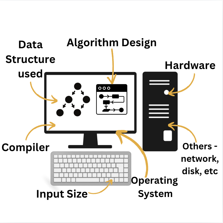
1. The size of the input data directly affects the running time of an algorithm. Larger inputs generally require more processing time.

2. The choice of data structure can significantly impact an algorithm's efficiency. 

   For example, using a hash table for searching can be much faster than a linear search.

3. The underlying logic and structure of an algorithm determine its efficiency. 

   Poorly designed algorithms may have bad time and space complexity.

4. Different programming languages have varying levels of performance and overhead. Some languages may be better suited for certain types of algorithms than others.

5. The processor speed, memory, and other hardware components of the system can influence an algorithm's execution time.

6. The compiler used to translate the code into machine instructions can affect performance through optimizations like loop unrolling, inlining, and constant folding.

7. The operating system can impact performance through factors such as process scheduling, memory management, and I/O operations.

8. Network latency, disk I/O, and other external factors can influence the overall execution time of an algorithm.

By understanding these factors, you can make informed decisions about algorithm selection and optimization to improve the performance of your applications.

Space Complexity measures the amount of memory an algorithm requires to execute as a function of the input size. This includes the memory used for variables, data structures, and function calls.

Time Complexity measures the amount of time an algorithm takes to execute as a function of the input size. It is typically expressed using Big O notation, which represents the upper bound on the growth rate of the algorithm's running time.

• Space and time complexity are often interrelated. Improving one may sometimes come at the expense of the other.

• The choice of data structures and algorithms can significantly impact both space and time complexity.

• It's important to analyze both space and time complexity to get a complete picture of an algorithm's performance.

Why are Space and Time Complexity Important?

1. Performance Optimization: Understanding space and time complexity helps you identify bottlenecks in your algorithms and optimize them for better performance.

2. Resource Allocation: Knowing the space and time requirements of an algorithm allows you to allocate appropriate resources for execution.

3. Scalability: Evaluating space and time complexity helps you assess how an algorithm will perform with larger input sizes, ensuring it can handle growth.

4. Algorithm Comparison: Comparing the space and time complexity of different algorithms can help you choose the most suitable one for a given task.

Big O notation provides a mathematical way to express the upper bound on an algorithm's execution time as the input size increases.

Big O notation focuses on the dominant term in the time complexity function.

• Common Big O complexities include:

  • O(1): Constant time (e.g., accessing an element in an array) -

    when algorithm is not dependent on the input size n

  • O(log n): Logarithmic time (e.g., binary search) -

    when algorithm reduces the size of the input data in each step.

  • O(n): Linear time (e.g., iterating over a list) -

    running time increases linearly with the length of the input

  • O(n log n): Log-linear time (e.g., merge sort) -

    similar to log time but runs for the input length

  • O(n^m): Quadratic time (e.g., nested loops) -

    running time increases non-linearly with increase in input, polynomial time complexity functions

Calculating Time Complexity

To calculate the time complexity of an algorithm, you can analyze the number of operations it performs as a function of the input size. This can be done by:

• Identify Basic Operations: Determine the fundamental operations performed by the algorithm, such as assignments, comparisons, and arithmetic operations.

• Assign Costs: Assign a cost to each basic operation. For simplicity, assume a constant cost (e.g., 1 unit of time) for each operation.

• Count Operations: Count the number of times each basic operation is executed as a function of the input size (n).

• Determine Dominant Term: Identify the term with the highest exponent in the resulting expression. This term will dominate the growth rate as n increases.

• Express in Big O Notation: Drop constant factors and lower-order terms to obtain the final time complexity expression in Big O notation.

Example:

Consider the following simple algorithm to find the maximum element in an array:

[Python]

def find_max(arr):
    max_val = arr[0]
    for num in arr:
        if num > max_val:
            max_val = num
    return max_val

• Basic Operations: Comparison (n-1 times), assignment (n times)

• Cost Function: Let's assume each operation takes constant time (C).

• Total Cost: T(n) = C(n-1) + C(n) = 2Cn - C

• Dominant Term: The dominant term is 2Cn.

• Time Complexity: O(n) (linear time)

  
  

Best-case, worst-case, and average-case analysis: 

Imagine you're racing a car, sometimes you're on a smooth, open road (best case), and sometimes you're stuck in traffic (worst case). But most of the time, you're somewhere in between (average case).

• Best-case: This is like winning a race. It's the fastest an algorithm can possibly run. Think of finding the first item in a list.

• Worst-case: This is like getting stuck in a traffic jam. It's the slowest an algorithm can run. Imagine searching for the last item in a list.

• Average-case: This is the most realistic scenario. It's like your usual commute. It's somewhere between the best and worst cases.

Different scenarios can affect an algorithm's performance. Analyzing these cases can provide a more complete understanding of its time complexity.

Interview Questions:

What is Big O notation and why is it important in algorithm analysis?

Big O notation is a mathematical tool used to describe the limiting behavior of a function as its argument tends towards a particular value or infinity. In computer science, it's primarily used to analyze the performance of algorithms, specifically their running time and space complexity. Big O notation is a valuable tool for analyzing algorithms, but it's important to consider other factors like the specific hardware and input data when evaluating an algorithm's overall performance.

Can you explain the difference between best-case, worst-case, and average-case time complexity?

Why is it important to analyze all three cases?

• Guarantees: Worst-case analysis provides a guarantee on the maximum running time of the algorithm, which is often crucial in real-world applications.

• Benchmarking: Comparing the best-case, worst-case, and average-case time complexities can help you benchmark different algorithms and choose the most appropriate one for a given task.

• Understanding limitations: Identifying the worst-case scenarios can help you optimize your algorithm or consider alternative approaches. Example:

  Consider the bubble sort algorithm.

  • Best-case: If the array is already sorted, bubble sort will complete in O(n) time (linear time).

  • Worst-case: If the array is sorted in reverse order, bubble sort will take O(n^2) time (quadratic time).

  • Average-case: The average-case time complexity of bubble sort is also O(n^2).

  By analyzing these different cases, you can get a better understanding of bubble sort's performance characteristics and make informed decisions about its use in your applications.

What are some common Big O notations and their implications for algorithm performance?

Big O provides a standardized way to compare the efficiency of different algorithms. Here are some common Big O notations and their implications:

1. Constant time (O(1)):

• The algorithm's running time remains the same regardless of the input size.

• Examples: Accessing an element in an array, simple arithmetic operations.

• Implication: Highly efficient for large datasets.

2. Linear time (O(n)):

• The running time increases linearly with the input size.

• Examples: Iterating over an array, simple searching algorithms.

• Implication: Suitable for smaller datasets, but can become inefficient for large inputs.

3. Logarithmic time (O(log n)):

• The running time increases logarithmically with the input size.

• Examples: Binary search, divide-and-conquer algorithms.

• Implication: Very efficient for large datasets, especially when the algorithm can repeatedly halve the input size.

4. Quadratic time (O(n^2)):

• The running time increases quadratically with the input size.

• Examples: Nested loops, brute-force algorithms.

• Implication: Can become inefficient for even moderately sized datasets, often indicating the need for optimization.

5. Exponential time (O(2^n)):

• The running time grows exponentially with the input size.

• Examples: Brute-force algorithms for certain problems like traveling salesman.

• Implication: Generally impractical for large datasets due to the rapid growth in running time.

Explain the significance of Big O notation in algorithm analysis

• Algorithm Comparison: Big O notation allows you to directly compare the efficiency of different algorithms for a given problem. 

• Performance Prediction: By understanding the Big O notation of an algorithm, you can predict how its performance will scale as the input size grows. This helps you make informed decisions about algorithm selection and optimization.

• Resource Allocation: Knowing the time complexity of an algorithm allows you to estimate the computational resources required to execute it. This helps you allocate resources effectively and avoid performance bottlenecks.

• Scalability: Big O notation is essential for understanding an algorithm's scalability. It helps you determine whether an algorithm can handle large datasets without significant performance degradation.

• Problem-Solving: By analyzing the time complexity of different approaches to a problem, you can identify more efficient solutions and avoid brute-force methods that may be impractical for large inputs.

Which algorithm would you choose for a task that requires searching a large dataset? Why?

1. Sorted Data:

• Binary Search: This algorithm is highly efficient for searching sorted arrays or lists. It works by repeatedly dividing the search interval in half until the target element is found or the interval becomes empty.

  • Time complexity: O(log n)

2. Unsorted Data:

• Linear Search: This is a simple but less efficient algorithm that sequentially iterates through the elements of the dataset until the target element is found.

  • Time complexity: O(n)

• Hash Table: If you need to perform frequent lookups and insertions, a hash table can be a good choice. It provides O(1) average-case time complexity for search and insertion operations.

  • Time complexity: O(1) (average case)

    
    

Factors to Consider:

• Data Distribution: If the data is uniformly distributed, a hash table might be more efficient. If the data is skewed, a different approach might be better.

• Frequency of Updates: If you need to frequently insert or delete elements, a data structure that supports efficient updates, such as a balanced binary search tree, might be preferable.

• Space Constraints: Consider the memory requirements of different algorithms. Some algorithms, like hash tables, may require additional space to store the data structure.

[ADV] How would you optimize an algorithm with a high time complexity?

Optimizing algorithms with high time complexity is essential for improving performance and ensuring scalability. Here are some strategies to consider:

1. Choose Appropriate Data Structures:

• Hash Tables: Efficient for searching and insertion operations.

• Trees: Well-suited for sorted data and range queries.

• Graphs: Useful for representing relationships between entities.

• Consider the trade-offs between space and time complexity when selecting data structures.

2. Divide and Conquer:

• Break down problems into smaller subproblems.

• Solve the subproblems recursively.

• Combine the solutions to solve the original problem.

• Examples: Merge sort, quicksort, binary search.

3. Dynamic Programming:

• Store intermediate results to avoid redundant calculations.

• Identify overlapping subproblems.

• Use memoization or tabulation to store and reuse results.

• Examples: Fibonacci sequence, matrix chain multiplication.

4. Greedy Algorithms:

• Make locally optimal choices at each step.

• May not always find the global optimal solution.

• Useful for problems like Dijkstra's algorithm and Huffman coding.

5. Branch and Bound:

• Explore the search space systematically.

• Prune branches that cannot lead to a better solution.

• Effective for optimization problems like the traveling salesman problem.

6. Algorithm-Specific Optimizations:

• For sorting algorithms: Consider hybrid approaches like Timsort or Introsort.

• For graph algorithms: Explore techniques like topological sorting or Dijkstra's algorithm.

• For string algorithms: Use specialized algorithms like KMP or Rabin-Karp for pattern matching.

7. Profiling and Benchmarking:

• Use profiling tools to identify performance bottlenecks.

• Measure the impact of optimizations on the algorithm's running time.

• Compare different algorithms and implementations.

Remember: There is no one-size-fits-all solution for optimizing algorithms. The best approach depends on the specific problem, the available data, and the desired performance goals. By carefully considering these factors and applying appropriate optimization techniques, you can significantly improve the efficiency of your algorithms.

[ADV] Explain the trade-offs between time complexity and space complexity.

Time complexity and space complexity are two fundamental metrics used to evaluate the performance of algorithms. While both are important, there is often a trade-off between them, meaning that improving one can sometimes lead to a decrease in the other. Here are some common trade-offs between time and space complexity:

• Sorting algorithms:

  • Merge sort: Has a good balance of time and space complexity, with O(n log n) for both.

  • Quick sort: Can be faster than merge sort in practice, but has a worst-case time complexity of O(n^2).

  • Insertion sort: Has a good space complexity of O(1) but can be slow for large datasets.

• Data structures:

  • Hash tables: Offer fast lookup and insertion times (O(1) on average), but can have a high space complexity if the load factor is low.

  • Arrays: Have a low space complexity but can be inefficient for certain operations like insertions and deletions.

  • Linked lists: Flexible data structures that allow for efficient insertions and deletions, but can have a higher space overhead than arrays.

• Algorithm design:

  • Brute-force algorithms: Often have high time complexity but may be simple to implement.

  • Divide-and-conquer algorithms: Can reduce time complexity but may require additional space for recursive calls.

  • Dynamic programming: Can improve time complexity by avoiding redundant calculations, but may require additional space to store intermediate results.

When is it appropriate to use a brute-force approach versus a more efficient algorithm?

Brute-force algorithms are straightforward and simple to implement, but they often have high time complexity. This means they can be inefficient for large datasets. However, there are situations where a brute-force approach might be appropriate:

• Small datasets: When the input size is relatively small, a brute-force algorithm might be sufficient.

• Quick prototyping: Brute-force algorithms can be used to quickly prototype a solution and test its feasibility before optimizing it.

• Guaranteeing correctness: Brute-force algorithms can guarantee that they will find the correct solution, even if they are inefficient.

When to consider a more efficient algorithm:

• Large datasets: If you're dealing with large amounts of data, a brute-force approach may be too slow. You'll need to consider more efficient algorithms with lower time complexity.

• Performance requirements: If your application has strict performance requirements, you'll need to choose algorithms that are optimized for speed.

• Scalability: If you anticipate the input size to grow significantly in the future, you'll need to choose algorithms that can handle large datasets efficiently.

How does the choice of data structure (e.g., array, linked list, hash table) impact the time complexity of algorithms?

• Access patterns: Consider how frequently you need to access elements randomly or sequentially.

• Insertion/deletion frequency: If you frequently need to add or remove elements, choose a data structure that supports efficient updates.

• Space requirements: Be mindful of the memory overhead associated with different data structures.

• Trade-offs: There are often trade-offs between time complexity and space complexity. Choose the data structure that best balances your needs.

  
  

• Here's a breakdown of how common data structures affect time complexity:

1. Arrays:

• Access: O(1) (constant time) for random access.

• Insertion/Deletion: O(n) (linear time) in the middle or at the end of the array, O(1) at the beginning.

  
  

2. Linked Lists:

• Access: O(n) (linear time) for random access.

• Insertion/Deletion: O(1) at the beginning or end of the list, O(n) in the middle.

  
  

3. Stacks and Queues:

• Access: O(1) for top/front element.

• Insertion/Deletion: O(1) for pushing/enqueuing, O(n) for removing elements from the middle.

  
  

4. Hash Tables:

• Search, insertion, deletion: O(1) on average.

• Worst-case: O(n) if there are many collisions.

  
  

5. Trees:

• Binary Search Trees:

  • Search, insertion, deletion: O(log n) in the average case, O(n) in the worst case.

• Balanced Binary Search Trees (e.g., AVL trees, red-black trees):

  • Search, insertion, deletion: O(log n) in all cases.

• Heaps:

  • Insertion/deletion: O(log n).

  • Finding the minimum/maximum: O(1).

Explain the concept of divide-and-conquer and its impact on time complexity.

Divide: Break the problem into smaller subproblems of the same type.

Conquer: Solve the subproblems recursively.

Combine: Combine the solutions of the subproblems to obtain the solution to the original problem.

The time complexity of divide-and-conquer algorithms depends on the number of subproblems created and the time complexity of solving each subproblem. In many cases, divide-and-conquer algorithms can achieve a time complexity of O(n log n), which is significantly better than brute-force approaches.

Examples of Divide-and-Conquer Algorithms:

• Merge sort: A sorting algorithm that divides the array into halves, recursively sorts each half, and then merges the sorted halves.

• Quick sort: Another sorting algorithm that partitions the array into two subarrays and recursively sorts each subarray.

• Binary search: A search algorithm that divides the search space in half at each step until the target element is found.

  
  

Advantages of Divide-and-Conquer:

• Reduced problem size: By breaking down problems into smaller subproblems, divide-and-conquer can make problems easier to solve.

• Improved efficiency: In many cases, divide-and-conquer algorithms can achieve significantly better time complexity than brute-force approaches.

• Parallelism: Divide-and-conquer algorithms can often be parallelized, allowing for faster execution on multi-core processors.

Can you describe the time complexity of common graph algorithms like breadth-first search (BFS) and depth-first search (DFS)?

Breadth-First Search (BFS):

• Time complexity: O(V + E), where V is the number of vertices and E is the number of edges in the graph.   

• Explanation: BFS explores vertices level by level, so it visits all vertices within a distance k from the starting vertex before moving to vertices at distance k+1. This results in a time complexity proportional to the sum of vertices and edges.

  
  

Depth-First Search (DFS):

• Time complexity: O(V + E)

• Explanation: DFS explores as deeply as possible along a path before backtracking. While the exact time complexity can vary depending on the implementation and the structure of the graph, it is generally O(V + E) in most cases.

  
  

Key points to remember:

• Both BFS and DFS have the same worst-case time complexity of O(V + E).

• The choice between BFS and DFS depends on the specific problem and the desired properties of the search algorithm.

• For example,

  BFS is often used to find the shortest path in unweighted graphs,

  while

  DFS can be used for topological sorting and detecting cycles.

[ADV] How can you identify bottlenecks in an algorithm and optimize its performance?

Bottlenecks are the parts of an algorithm that consume the most resources (time or space). Identifying and optimizing these bottlenecks can significantly improve an algorithm's overall performance.

Here are some strategies to identify and optimize bottlenecks:

1. Profiling:

• Use profiling tools: Tools like Python's cProfile or Java's VisualVM can help you measure the execution time of different parts of your code.

• Identify hot spots: Look for functions or code sections that take up the most time.

2. Algorithm Analysis:

• Review time complexity: Analyze the algorithm's Big O notation to identify potential bottlenecks.

• Consider data structures: Evaluate if using different data structures can improve performance.

• Optimize recursive algorithms: Look for opportunities to convert recursive algorithms to iterative ones to reduce function call overhead.

3. Memory Management:

• Reduce memory usage: Optimize data structures and avoid unnecessary memory allocations.

• Use memory-efficient algorithms: Consider algorithms that have lower space complexity.

4. Input/Output (I/O) Operations:

• Minimize I/O: Reduce the number of read/write operations to disk or network.

• Use caching: Store frequently accessed data in memory to reduce I/O overhead.

5. Compiler Optimizations:

• Enable compiler optimizations: Many compilers have built-in optimizations that can improve performance.

• Review compiler output: Analyze the generated assembly code to identify potential bottlenecks.

6. Parallel Processing:

• Explore parallelization: If your algorithm can be parallelized, consider using multiple cores or threads to improve performance.

7. Benchmarking:

• Measure performance: Conduct benchmarks to compare different implementations and identify the most efficient approach.

• Iterative Refinement: Continuously measure and optimize performance as you make changes to your code.

What strategies can be used to reduce the time complexity of recursive algorithms?

Recursive algorithms can be powerful tools, but they can also lead to high time complexity if not optimized carefully. 

Here are some strategies to reduce the time complexity of recursive algorithms:

1. Memoization:

• Store intermediate results: Store the results of function calls in a cache or table.

• Avoid redundant calculations: If the same subproblem is encountered again, retrieve the result from the cache instead of recalculating it.

• Example: Fibonacci sequence with memoization can significantly reduce time complexity. (dynamic programming)

2. Tail Recursion Optimization:

• Convert tail-recursive functions to iterative equivalents: Tail-recursive functions are those where the recursive call is the last operation performed in the function. Compilers can often optimize tail-recursive functions into iterative loops, reducing stack space usage and improving performance.

3. Divide-and-Conquer Optimization:

• Choose appropriate subproblem sizes: Ensure that the subproblems are of roughly equal size to avoid unbalanced recursion trees.

• Optimize the combination step: Find efficient ways to combine the solutions of the subproblems.

4. Early Termination:

• Identify conditions where the recursion can terminate early. This can help reduce the number of recursive calls and improve performance.

5. Iterative Implementation:

• If possible, convert the recursive algorithm to an iterative one. This can often eliminate the overhead of function calls and reduce stack space usage.

[ADV] How can you trade off space complexity for improved time complexity in certain scenarios?

In many cases, there is a trade-off between time complexity and space complexity. Improving one often comes at the expense of the other. This means that you may need to sacrifice memory usage to achieve faster execution times, or vice versa.

Strategies for Trading Off Space for Time:

1. Caching:

   • Store frequently accessed data in memory: This can reduce the number of expensive lookups, improving time complexity.

   • Trade-off: Increased space usage to store the cached data.

2. Memoization:

   • Store intermediate results to avoid redundant calculations: This can significantly improve time complexity, especially for recursive algorithms.

   • Trade-off: Increased space usage to store the memoization table.

3. Data Structures:

   • Choose data structures that prioritize time complexity over space: For example, using a hash table for fast lookups might require more memory than a linked list.

   • Consider space-efficient alternatives: Explore data structures that have lower space requirements, even if they might have slightly higher time complexity.

4. Algorithm Design:

   • Explore algorithms with different time-space trade-offs: Some algorithms may be faster but require more memory, while others may be slower but use less memory.

   • Consider the specific requirements of your application: If memory is a critical constraint, you may need to prioritize space efficiency over time complexity.

Example:

In graph algorithms, using depth-first search (DFS) might require less space than breadth-first search (BFS), but BFS can sometimes be faster. The choice between the two depends on the specific problem and the available resources.

Key Considerations:

• Input size: For small datasets, space complexity may be less of a concern. However, for large datasets, optimizing space usage can be crucial.

• Performance requirements: If real-time performance is critical, you may need to prioritize time complexity over space complexity.

• Memory constraints: If you are working with limited memory resources, you may need to focus on optimizing space complexity.

Extra Questions for you to try out !

• Compare the time complexities of bubble sort and merge sort.

• Given a code snippet, can you determine its time complexity?

• What is the time complexity of bubble sort, merge sort, and quicksort?

• Given a specific problem, can you design an efficient algorithm and analyze its time complexity?

  
  

Resources:

https://www.mygreatlearning.com/blog/why-is-time-complexity-essential

Online Courses and Tutorials:

• Coursera: Offers courses on algorithms and data structures by top universities.

• LeetCode: Provides a vast collection of coding problems with solutions and difficulty levels.

• HackerRank: Offers practice problems, challenges, and contests to improve your skills.

• GeeksforGeeks: A comprehensive resource with articles, tutorials, and practice problems on various data structures and algorithms.